![[데이터 분석] 모델 성능 향상](https://img1.daumcdn.net/thumb/R750x0/?scode=mtistory2&fname=https%3A%2F%2Fblog.kakaocdn.net%2Fdn%2Fc3tNFV%2FbtrPK1aaVRU%2FiBZ0gyauWRArv9jHD4JVZ0%2Fimg.png)

[데이터 분석] 모델 성능 향상Data Analysis2022. 10. 28. 00:32
Table of Contents
반응형
모델 성능 향상에는 다음과 같은 방법들이 존재합니다! 저같은 경우는 빠르게 분석하기 위해 3개의 방법을 이용하는데요!
1. 모델 하이퍼 파라미터 튜닝
2. Coef를 통해 영향이 큰 피처 이상치 제거
3. 모델 앙상블 (보팅/스태킹)
1. Hyper Params Tuning
Gridsearch 를 이용해 최적의 하이퍼파라미터를 찾는다. 엔지니어링하는 것 보다 최적의 파라미터를 구할 수 있는 장점이 있지만 찾는 데 오래걸리는 단점이 있다.
gb_reg = GradientBoostingRegressor()
gb_reg.get_params().keys() # 모델 파라미터 확인
#Regressor : Gradient Boosting Regressor
params = {'n_estimators': [200,400],
'learning_rate': [0.1, 0.05, 0.01],
'max_depth': [5, 10],
'min_samples_leaf': [100,150],
'max_features': [0.3, 0.1]
}
grid_gb = GridSearchCV(gb_reg, param_grid=params, cv=5, scoring='neg_mean_squared_error', verbose=4)
grid_gb.fit(X_features, y_feature)
gb_best = grid_gb.best_estimator_
#cls : scoring = 'accuracy'#classifier
params = {
'n_estimators':[100],
'max_depth' : [6, 8, 10, 12],
'min_samples_leaf' : [8, 12, 18],
'min_samples_split' : [8, 16, 20]
}
# RandomForestClassifier 객체 생성 후 GridSearchCV 수행
rf_clf = RandomForestClassifier(random_state=0, n_jobs=-1)
grid_cv = GridSearchCV(rf_clf , param_grid=params , cv=2, n_jobs=-1 )
grid_cv.fit(X_train_over, y_train_over)
print('최적 하이퍼 파라미터:\n', grid_cv.best_params_)
print('최고 예측 정확도: {0:.4f}'.format(grid_cv.best_score_))2. Coef 영향이 큰 피처 이상치 제거
model.coef_ 되는 모델은 linear 모형만 가능하다. (linear regression, lasso, ridge)
def get_top_bottom_coef(model):
    # coef_ 속성을 기반으로 Series 객체를 생성. index는 컬럼명.
    coef = pd.Series(model.coef_, index=X_feature.columns)

    # + 상위 10개 , - 하위 10개 coefficient 추출하여 반환.
    coef_high = coef.sort_values(ascending=False).head(10)
    coef_low = coef.sort_values(ascending=False).tail(10)
    return coef_high, coef_low
def visualize_coefficient(models):
# 3개 회귀 모델의 시각화를 위해 3개의 컬럼을 가지는 subplot 생성
fig, axs = plt.subplots(figsize=(24,10),nrows=1, ncols=3)
fig.tight_layout()
# 입력인자로 받은 list객체인 models에서 차례로 model을 추출하여 회귀 계수 시각화.
for i_num, model in enumerate(models):
# 상위 10개, 하위 10개 회귀 계수를 구하고, 이를 판다스 concat으로 결합.
coef_high, coef_low = get_top_bottom_coef(model)
coef_concat = pd.concat( [coef_high , coef_low] )
# 순차적으로 ax subplot에 barchar로 표현. 한 화면에 표현하기 위해 tick label 위치와 font 크기 조정.
axs[i_num].set_title(model.__class__.__name__+' Coeffiecents', size=25)
axs[i_num].tick_params(axis="y",direction="in", pad=-120)
for label in (axs[i_num].get_xticklabels() + axs[i_num].get_yticklabels()):
label.set_fontsize(22)
sns.barplot(x=coef_concat.values, y=coef_concat.index , ax=axs[i_num])
models = [lr, rid, las]

#visualize_coefficient(models)
get_top_bottom_coef(rid)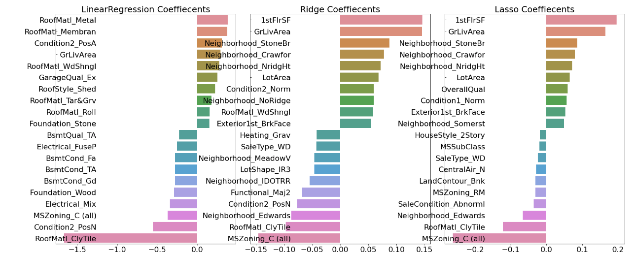
# 이상치 제거 : 1stFlrSF, GrLivArea 피처의 coef가 높기 때문에 영향을 주는 이상치 제거

plt.scatter(x = train_ori['1stFlrSF'], y=train_ori['SalePrice'])

cond1 = train_ohe['GrLivArea'] > np.log1p(4000)
cond2 = train_ohe['GrLivArea'] < np.log1p(500000)
outlier_idx = train_ohe[cond1 & cond2].index

print('이상치 제거 전 : {0}'.format(train_ohe.shape))

train_ohe.drop(outlier_idx, inplace=True)
print('이상치 제거 후 : {0}'.format(train_ohe.shape))
3. 모델 앙상블
Voting
- 하드 보팅 : 각 classifier의 결과값을 다수결로 결정. e,g, [1], [1], [1], [0] -> 최종 결과 [1]
- 소프트 보팅 : 다수의 classifier의 class 확률을 평균하여 결정.
- e.g. [1일 확률 : 0.6 , 0일 확률 : 0.4] , [1일 확률 : 0.7 , 0일 확률 : 0.3] .. -> 평균하여 최종결과 [1일 확률 : 0.65, 0일 확률 : 0.35]
from sklearn.ensemble import VotingClassifier

vo_clf = VotingClassifier(estimators=[('LR',lr_clf), ('RF', rf_clf)], voting='soft') #default = 'hard'
vo_clf.fit(X_train, y_train)
vo_pred = vo_clf.predict(X_test)

get_clf_eval(y_test, rf_pred)
728x90
반응형
'Data Analysis' 카테고리의 다른 글
| [데이터 분석] 라벨 불균형 처리 (0) | 2022.10.28 |
|---|---|
| [데이터 분석] 이상치 처리 (0) | 2022.10.28 |
| [데이터 분석] 선형회귀 / 다항회귀 (0) | 2022.10.26 |
@부지런깨꾹이 :: Gaegul's devlog
Action speaks louder than words. 하루 하루의 기록을 습관화 합니다 📖
포스팅이 좋았다면 "좋아요❤️" 또는 "구독👍🏻" 해주세요!
![[데이터 분석] 이상치 처리](https://img1.daumcdn.net/thumb/R750x0/?scode=mtistory2&fname=https%3A%2F%2Fblog.kakaocdn.net%2Fdn%2FHtw3z%2FbtrPJ4ZA2jh%2Ff481ElVW9SzJXujDVjJ5a0%2Fimg.png)
![[데이터 분석] 선형회귀 / 다항회귀](https://img1.daumcdn.net/thumb/R750x0/?scode=mtistory2&fname=https%3A%2F%2Fblog.kakaocdn.net%2Fdn%2FbwCsB2%2FbtrPB1JZvPL%2FY3kZ2Qt1VAfgwGyqYOL330%2Fimg.png)