[의료 이미지] CT image 이해하기 (feat. Dicom 파일)

논문을 읽기 앞서 CT image의 Dicom 파일과 뇌출혈 subtype에 관해 알아보겠습니다.

 

1.  Dicom 파일이란?

DICOM은 의학 분야의 Digital Imaging and Communications의 약자입니다. 초음파 및 MRI 이미지와 같은 의료 정보를 환자의 정보와 함께 하나의 Dicom 파일에 저장할 수 있습니다.

 

•  dicom 파일 여는 법 

pydicom libraray를 설치 후에 사용 할 수 있습니다. 데이터 안에는 다음과 같은 meta 정보가 포함되어 있습니다.

meta 정보에는 이미지 사이즈,  Window 사이즈, 환자 정보, Study Instance UID, Series Instance UID등이 포함되어 있습니다.

 

data = pydicom.read_file('/content/ID_000012eaf.dcm')

Dataset.file_meta -------------------------------
(0002, 0000) File Meta Information Group Length  UL: 188
(0002, 0001) File Meta Information Version       OB: b'\x00\x01'
(0002, 0002) Media Storage SOP Class UID         UI: CT Image Storage
(0002, 0003) Media Storage SOP Instance UID      UI: 1.2.840.4267.32.337944818669776895705763408052798539612
(0002, 0010) Transfer Syntax UID                 UI: Explicit VR Little Endian
(0002, 0012) Implementation Class UID            UI: 1.2.40.0.13.1.1.1
(0002, 0013) Implementation Version Name         SH: 'dcm4che-1.4.35'
-------------------------------------------------
(0008, 0018) SOP Instance UID                    UI: ID_000012eaf
(0008, 0060) Modality                            CS: 'CT'
(0010, 0020) Patient ID                          LO: 'ID_f15c0eee'
(0020, 000d) Study Instance UID                  UI: ID_30ea2b02d4
(0020, 000e) Series Instance UID                 UI: ID_0ab5820b2a
(0020, 0010) Study ID                            SH: ''
(0020, 0032) Image Position (Patient)            DS: [-125.000000, -115.897980, 77.970825]
(0020, 0037) Image Orientation (Patient)         DS: [1.000000, 0.000000, 0.000000, 0.000000, 0.927184, -0.374607]
(0028, 0002) Samples per Pixel                   US: 1
(0028, 0004) Photometric Interpretation          CS: 'MONOCHROME2'
(0028, 0010) Rows                                US: 512
(0028, 0011) Columns                             US: 512
(0028, 0030) Pixel Spacing                       DS: [0.488281, 0.488281]
(0028, 0100) Bits Allocated                      US: 16
(0028, 0101) Bits Stored                         US: 16
(0028, 0102) High Bit                            US: 15
(0028, 0103) Pixel Representation                US: 1
(0028, 1050) Window Center                       DS: "30.0"
(0028, 1051) Window Width                        DS: "80.0"
(0028, 1052) Rescale Intercept                   DS: "-1024.0"
(0028, 1053) Rescale Slope                       DS: "1.0"
(7fe0, 0010) Pixel Data                          OW: Array of 524288 elements

 

• Dicom 파일 이해하기

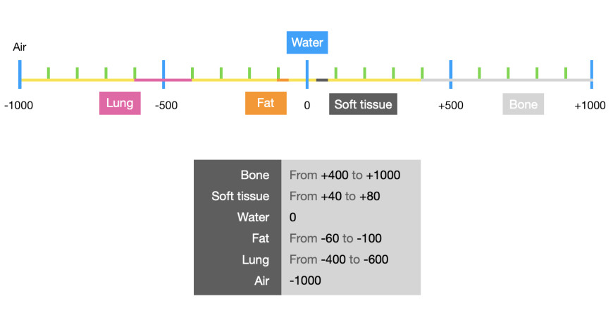
CT image의 픽셀 값은 일반 RGB 이미지와는 다릅니다. RGB 이미지의 각 픽셀은 0 ~ 255의 값으로 이루어져 있지만, CT는 Hounsfield Unit (HU)라는 단위로 이루어져 있습니다. 여기서 HU란 X 선이 몸을 투과할 때 감쇠되는 정도를 나타내는 단위입니다. 

 

조금 더 이해하기 쉽게 표를 가지고 왔는데 , 다음 그림은 물 = 0을 기준으로 각 부위의 HU 값을 나타내는 표입니다. 

 

CT 영상의 픽셀들은 HU 값으로 구성되어 있기 때문에 보고 싶은 신체 부위가 있다면 HU 표를 참고해  Window Center와 Window Width를 조절한 뒤에 그 부분 위주로 출력해줄 수 있습니다.

 

Window Center는 보고 싶은 부위의 HU 값을 의미하고, Window Width는 WC를 중심으로 관찰하고자 하는 HU 범위를 의미합니다.

 

그래서 만약 뼈를 보고 싶다고 하면, window center 와 width을 400과 1000으로 넣고 스케일링 해주면 뼈 부분이 더 잘 보이게 됩니다. 

[출처 : https://vincentblog.xyz/posts/medical-images-in-python-computed-tomography]

 

 

• Dicom 파일의 window 조정 code

# dicom 파일에서 각 value값들 가져오기

def get_window(data):
  dicom_fields = [data[('0028', '1050')].value, # Window Center 
                  data[('0028', '1051')].value, # Window Width 
                  data[('0028', '1052')].value, # Rescale Intercept
                  data[('0028', '1053')].value] # Rescale Slope

  return [get_first_of_dicom_field_as_int(x) for x in dicom_fields]

# 원하는 window값 넣어서 scaling 해주기

def window_image(img, window_center, window_width, intercept, slope, rescale=True):
  img = (img * slope + intercept)
  img_min = window_center - window_width//2
  img_max = window_center + window_width//2

  img[img<img_min] = img_min
  img[img>img_max] = img_max

  if rescale:
    img = (img-img_min) / (img_max - img_min)

    return img   

window_center, window_width, intercept, slope = get_window(data)
img = pydicom.read_file('/content/ID_000012eaf.dcm').pixel_array #array

# displaying the image : Three window
# Brain window : 40-80
# Subdural window : 80~200
# Bone window : 600~2800

fig, (ax1, ax2, ax3, ax4) = plt.subplots(4,1, sharex='col', figsize=(10,24), gridspec_kw={'hspace': 0.1, 'wspace': 0})

ax1.set_title('Default window')
im1 = ax1.imshow(img,  cmap=plt.cm.bone)

ax2.set_title('Brain window') # Brain window 
img2 = window_image(img, 40, 80, intercept, slope)
im2 = ax2.imshow(img2, cmap=plt.cm.bone)

ax3.set_title('Subdural window') 
img3 = window_image(img, 80, 200, intercept, slope) # Blood/Subdural window 
im3 = ax3.imshow(img3, cmap=plt.cm.bone) 
# ax3.annotate('', xy=(150, 380), xytext=(120, 430),
#             arrowprops=dict(facecolor='red', shrink=0.05),
#             )
# ax3.annotate('', xy=(220, 430), xytext=(190, 500),
#             arrowprops=dict(facecolor='red', shrink=0.05),
#             )

ax4.set_title('Bone window')
img4 = window_image(img, 600, 2800, intercept, slope) # Bone window 
im4 = plt.imshow(img4, cmap=plt.cm.bone)

for ax in fig.axes:
    ax.axis("off")
    
plt.show()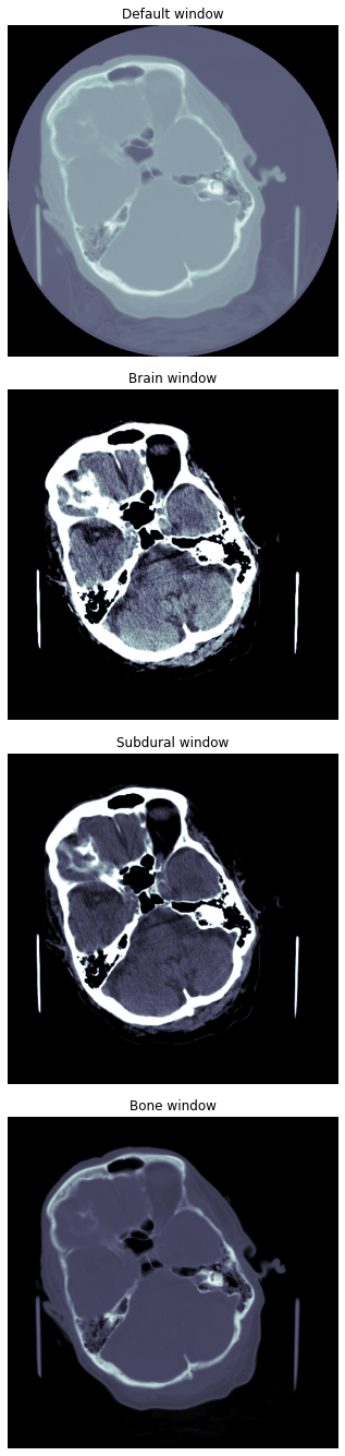

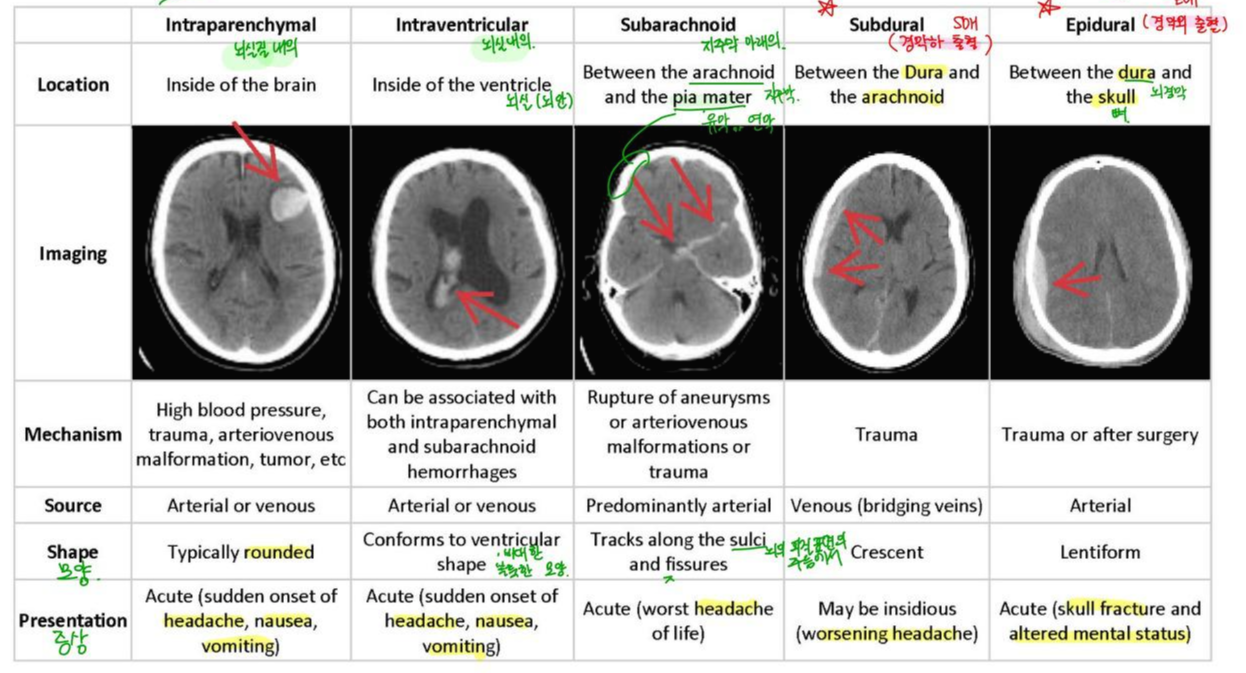
window 별 출력 이미지 

 

 

2.  뇌출혈 5가지 Subtypes  

1. cerebral parenchymal Hemorrhage(CPH) : 뇌 안에 생기는 출혈. 
2. intraventricular Hemorrhage(IVH) :  뇌실 안에 생기는 출혈. 
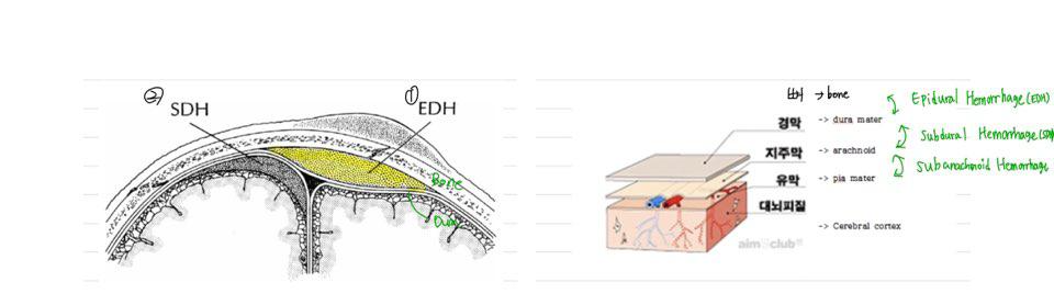
3. subarachnoid Hemorrhage(SAH)  : 지주막(arachnoid) 과 연막(pia mater) 사이에서 생기는 출혈
4. subdural Hemorrhage(SDH) : 경막(dura)와 지주막(arachnoid) 사이에서 생기는 출혈.
5. epidural Hemorrhage(EDH) : 경막(dura)와 뼈 사이에 생기는 출혈.

*뇌실 : 뇌 사이의 빈 공간.

 

[ 각 뇌출혈 종류의 특징들 ] 

출처 : Kaggle - RNSA intracranial-hemorrhage-detection

 

제가 공부하면서 필기해논 그림입니다.

각 뇌출혈 위치, 이미지, 모양, 증상을 설명하고 있으니 참고 하실 분들은 참고하세요 :)

(왼쪽) SDH 와 EDH 위치 (오른쪽) EDH , SDH, EDH 위치 단면